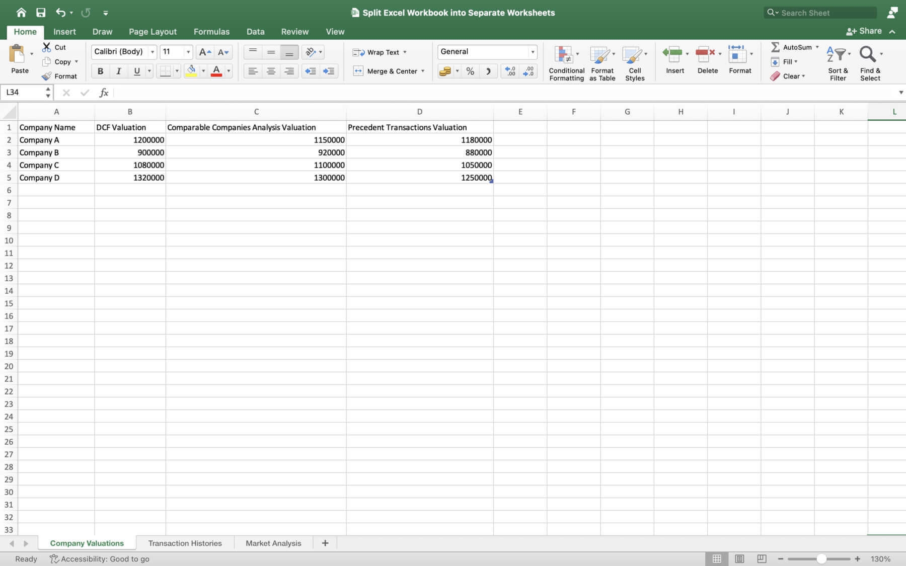
Excel is a powerful tool for organizing and analyzing data. One useful feature in Excel is the ability to link worksheets, allowing you to easily reference data from one sheet to another. This can be especially helpful when working with large datasets or when creating complex formulas.
By linking worksheets in Excel, you can streamline your workflow and ensure that your data is accurate and up to date across all sheets. In this article, we will discuss how to link worksheets in Excel and provide some tips for effectively using this feature.
Steps to Link Worksheets in Excel
1. Open the Excel workbook that contains the worksheets you want to link. Click on the tab of the worksheet where you want to create the link.
2. Select the cell where you want the linked data to appear. Type an equal sign (=) in the cell to start a formula.
3. Click on the tab of the worksheet that contains the data you want to link to. Select the cell or range of cells that you want to link.
4. Press Enter to complete the formula and link the data from the other worksheet. The linked data will now appear in the cell you selected on the first worksheet.
5. To update the linked data, simply make changes to the original data on the other worksheet. The linked data will automatically update to reflect the changes.
By following these steps, you can easily link worksheets in Excel and create dynamic connections between your data. This can save you time and reduce the risk of errors when working with multiple sheets of data.
In conclusion, linking worksheets in Excel is a valuable feature that can help you organize and analyze your data more effectively. By following the steps outlined in this article, you can easily create links between worksheets and ensure that your data is accurate and up to date. Incorporating this feature into your Excel workflow can improve your productivity and make working with large datasets more manageable.
